What Makes a Good 4D STEM Dataset?
A 30-minute read
Acquisition Choices Before Reconstruction
4D STEM acquires a diffraction pattern at every probe position as the electron beam is scanned across the specimen. An overview of the method and its principal applications is given in [1].
The question of what constitutes a good 4D STEM dataset has no single answer, and it depends on the intended analysis. A dataset suitable for virtual bright-field imaging is not necessarily suitable for ptychography, and a dataset for strain mapping would be poorly suited to differential phase contrast. The acquisition strategy must be chosen with the downstream analysis in mind.
This article discusses several common 4D STEM applications and the acquisition parameters that affect dataset quality for each. A broader survey of techniques enabled by 4D STEM is also given in [1].
Setting acquisition parameters begins with a single question:
What information must the dataset contain for the intended analysis?
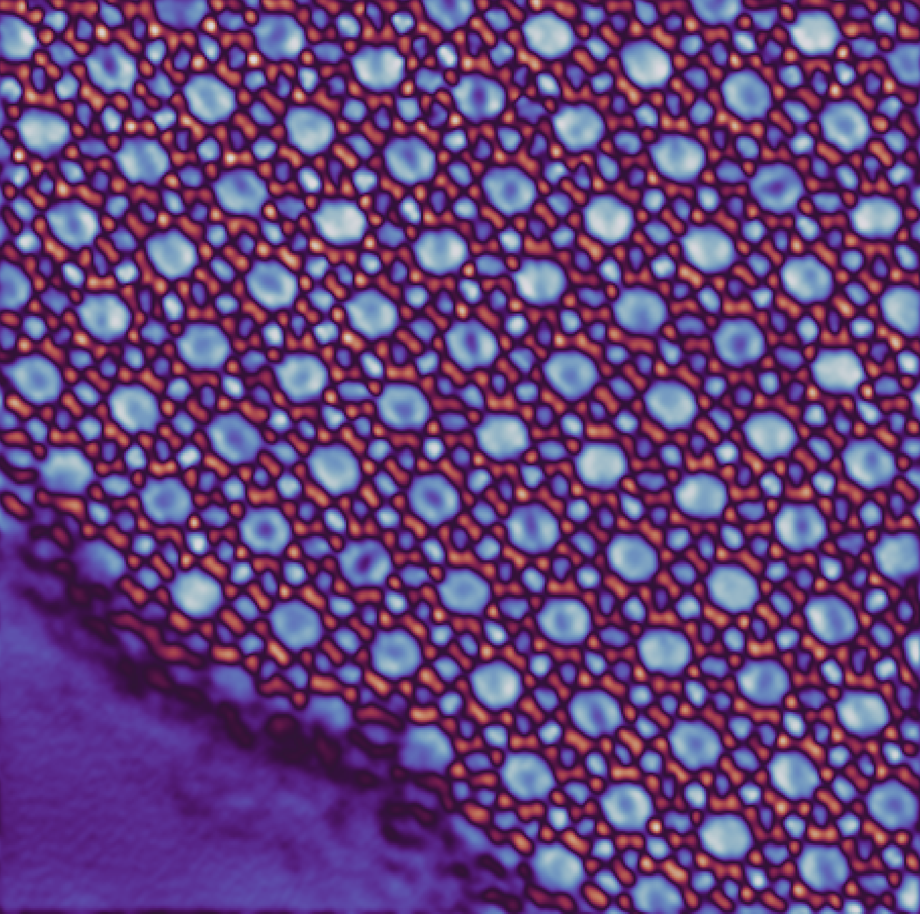
Figure 1: 4D STEM ptychographic reconstruction of a zeolite material. Data acquired with QUADRO and Novena Acquire. Image credit: Yujiao Wang and Daliang Zhang (Chongqing University); Qingxiao Wang, Cailing Chen, and Yiqiang Chen (KAUST).
Acquisition Strategy Depends on the Analysis
The choice of acquisition parameters follows from the intended analysis. Different analyses use different aspects of the recorded diffraction patterns and process them in different ways. What counts as a usable dataset therefore depends on how the dataset will be analyzed.
In virtual bright-field and dark-field imaging, images are formed by summing the detector counts within a chosen virtual aperture at each probe position. The recorded angular range must include the scattering angles selected by that virtual aperture. For strongly scattering materials, or for analyses that rely on higher-angle contrast, the recorded range must extend far enough to capture the relevant signal.
Center-of-mass (COM) and differential phase contrast (DPC) measure how the bright-field disk deflects across the scan. The measurement is the position of the disk centroid on the detector at each probe position. Small shifts encode local electric and magnetic fields in the sample. Because the disk position is the measurement, the disk must be centered on the detector, stable across the scan, and unsaturated.
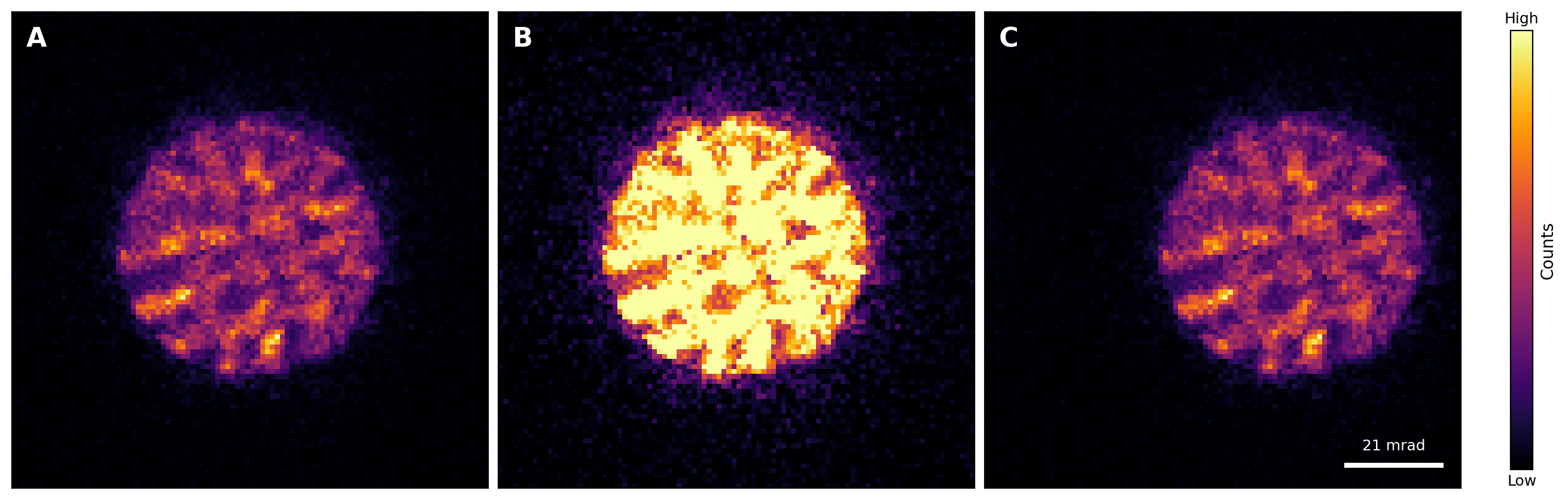
Figure 2: Possible diffraction pattern artefacts. (A) A reference diffraction pattern from [2], acquired with a convergence semi-angle of 27.6 mrad and a recorded angular range of 50.9 mrad. (B) The same pattern after digital thresholding to simulate detector saturation. Fine intensity variation within the bright-field disk is lost, which affects any analysis that relies on the content of the disk. (C) A non-centered diffraction pattern. Off-centering reduces the angular range available for analysis: after cropping to recenter the pattern, the maximum recorded angle drops to approximately 32 mrad, which imposes a corresponding limit on the resolution achievable in ptychography.
Strain mapping tracks Bragg disk positions across the scan to recover the local strain value. These methods are usually carried out over large fields of view. The smallest resolvable strain is set by how sharp and stable those Bragg features are.
Ptychography is usually more demanding on acquisition parameters, and it works differently from the others. The earlier methods extract a small set of values from each diffraction pattern (an integrated intensity, a centroid position, a Bragg disk position) and assemble those into a real-space map. Ptychography instead uses the diffraction patterns themselves as input to an iterative reconstruction that solves for the object, and often for the probe itself, using overlap between neighboring probe positions. The dataset must provide both real-space overlap and a well-sampled diffraction pattern. The next three sections look at each acquisition axis in more detail, with ptychography returning at the end as a case study.
Reciprocal-space sampling: the Camera-length Trade-off
At each probe position, the detector records only a finite region of reciprocal space, and magnification of the projector system, commonly referred to as camera length, is what sets the size of that window.
A shorter camera length records a wider range of scattering angles, with each pixel covering more reciprocal space, while a longer camera length narrows the range but samples it more finely. Neither end is universally preferable, and the right setting depends on the measurement.
The trade-off matters most for ptychography, where two distinct concerns are at stake. The maximum recorded angle sets a ceiling on the spatial resolution the reconstruction can reach, because the algorithm cannot recover information that was never on the detector. Separately, the sampling density within the recorded range determines whether the fine structure of the diffraction pattern is captured at all. This second concern is sharpest in iterative ptychography, where introducing defocus brings additional details into the diffraction pattern, and the detector has to sample those details with enough pixels to resolve them. At a given camera length, the detector's pixel size and array dimensions together set both the recorded angular range and the sampling density within it.
For the other methods, the camera-length requirements are simpler. Virtual bright-field and dark-field imaging need the intended collection angles to fall within the recorded range, and COM and DPC need the bright-field disk to stay on the detector face and remain centered. For strain mapping, the pixel-to-angle calibration sets a limit on the achievable strain precision.
Before acquisition, the detector configuration should be verified against the angular range and sampling density required by the intended analysis.
Signal quality: Dose, Dynamic range, and Saturation
In many 4D STEM experiments, the diffraction pattern contains an intense low-angle component and a much weaker scattered signal at higher angles. The dynamic range required to record both within a single frame is large. Overexposure saturates the bright-field disk, and if the detector has a noise floor or background, underexposure leaves the weaker features below it.
The harm caused by saturation depends on the analysis. For virtual dark-field imaging, saturation in the bright-field disk may have no effect on the result, but for COM, DPC, ptychography, and quantitative analyses in general, saturated pixels can render the diffraction pattern unusable. As a rule, the relevant signal must remain within the detector's working range.
The dose delivered to the specimen and the counts recorded per frame are set by the same handful of acquisition parameters: beam current, dwell time per probe position, and how densely the scan grid samples the specimen. These parameters interact. The same counts per frame can be reached at lower beam current with a longer dwell, or at higher current with a shorter dwell. Longer dwell extends acquisition time and increases sensitivity to drift, while higher current at a fixed dwell raises the instantaneous count rate on the detector and makes saturation more likely.
Beam-sensitive specimens introduce an additional constraint. In general, higher dose yields better counting statistics, but for beam-sensitive samples there is a threshold above which additional dose no longer improves the data. Beyond this threshold, the specimen begins to change, and in some cases is destroyed before the measurement is complete. For biological specimens, dose budgets are typically discussed in the range of a few tens of electrons per square ångström, although damage to high-resolution information can occur at lower doses [3]. For materials such as MOFs and COFs, the acceptable dose can be substantially lower than for most inorganic samples [4].
Detector performance can offset the effect of the above-mentioned trade-offs. A detector with high dynamic range can record strong and weak signals in the same frame, and electron-counting detection has no background noise, which matters most when the relevant signal is weak. Fast readout reduces sensitivity to drift and microscope instabilities, and enables techniques such as dose fractionation.
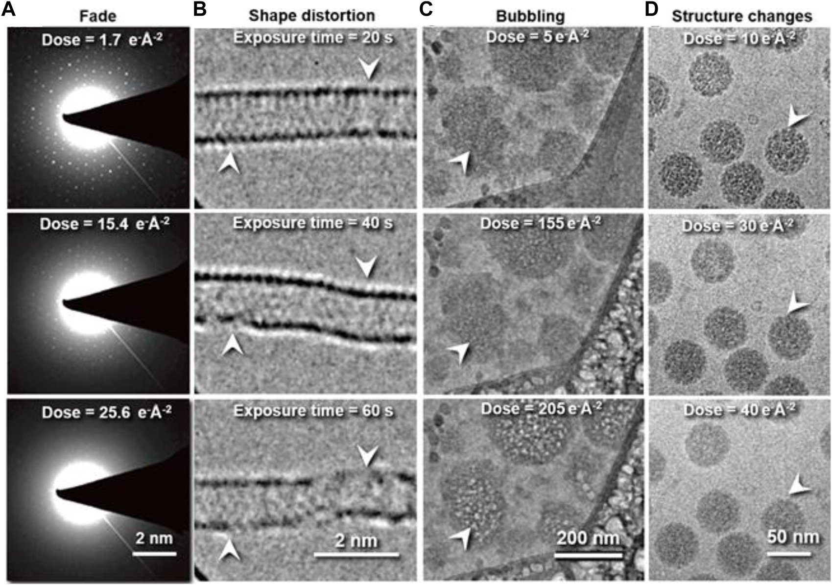
Figure 3: Beam-induced damage observed across different specimen types and modalities [5,6,7,8,9]. (A) Loss of high spatial frequencies in the diffraction domain as accumulated dose increases. (B) Specimen distortion, observed as changes in shape and dimension under continued exposure. (C) Bubble formation in biological samples under high accumulated dose. (D) Loss of fine detail in real-space imaging at increasing dose, the real-space view of the same effect shown in (A).
Real-space Sampling: Scan Grid and Scan Stability
The scan grid determines where on the specimen each diffraction pattern is recorded, and how densely those positions are spaced. For virtual bright-field, virtual dark-field, COM, and DPC imaging, the scan step directly sets the pixel size of the resulting image. The step has to be fine enough to sample any spatial feature the experiment intends to resolve, and finer steps come at the cost of more probe positions, longer total acquisition time, and larger datasets.
For methods such as tilt-corrected bright-field imaging and ptychography, the relationship between scan step and final pixel size is less direct, but the scan step remains critical. In ptychography, adjacent probe positions must overlap by a sufficient amount, and the overlap is determined jointly by the scan step, the convergence semi-angle, and the defocus condition. Scan parameters and microscope settings are therefore not independent.
The field of view is also a design choice. Orientation mapping needs an area large enough to contain the grains or domains of interest, while strain mapping needs to cover whatever spatial scale of strain matters for the measurement. The cost of a larger field of view is either a coarser scan step at fixed dataset size, or a larger dataset at fixed step.
The scan coils place the probe at the intended position on the specimen, and the descan coils keep the diffraction pattern centered on the detector as the probe moves. Sample drift moves the specimen under the probe, and scan distortion bends the probe trajectory away from the commanded grid. In drastic cases, this produces a warped real-space image. Descan misalignment, by contrast, leaves the probe correctly placed, but causes the diffraction pattern to move on the detector across the scan, and that shift becomes part of any quantity measured from the pattern. For example, a diffraction pattern that drifts during the scan may distort the resulting strain map.
Even when the scan is stable, the absolute scale of the recorded grid must be correct. The conversion from scan-coil current to physical distance on the specimen sets the accuracy of any real-space measurement made from the dataset, and the effect of mis-calibration depends on the analysis. For methods in which the scan step directly sets the pixel size of the resulting image (virtual bright-field, dark-field, COM, DPC), mis-calibration leads to wrong spatial scales in the final image. For ptychography, the reconstruction requires accurate probe positions, and a mis-calibrated step size can prevent it from converging to a correct reconstruction.
Scan stability and the signal integrity of the scan electronics are part of delivering a clean dataset, alongside the detector itself. DECTRIS supplies its detectors as part of a complete scanning pipeline, working with established scan-generator manufacturers. At installation, both the real-space pixel size and the reciprocal-space pixel size are calibrated, so the recorded scan grids and diffraction patterns correspond to the physical scales they represent.
Ptychography: Where the Acquisition Choices Come Together
In many 4D STEM analyses, imperfections in the dataset reduce the quality of the result but do not break it. Ptychography is less forgiving, because the reconstruction depends on multiple conditions being satisfied at once: a well-aligned microscope, sufficient overlap between neighboring probe positions, and well-sampled diffraction patterns. If any of these conditions fails, the reconstruction will not be reliable.
Alignment is particularly critical for ptychography. The algorithm assumes a specific probe shape and scan geometry as its starting point, and significant deviations from that model degrade the reconstruction. Modern algorithms can refine the probe iteratively, but they still need a reasonable starting estimate to converge.
No single parameter set is universally optimal. The right choice depends on the specimen and the experimental question. Two cases at opposite extremes illustrate this:
|
Case A: atomic-resolution materials [2] |
Case B: biological single-particle imaging [10] |
|
|
Convergence semi-angle |
27.6 mrad |
4.0 mrad |
|
Scan step size |
0.33 Å |
20.0 Å |
|
Field of view |
51 x 27 nm2 |
256 x 256 nm2 |
|
Defocus |
~20 nm |
~1.5 µm |
|
Max recorded angle |
50.9 mrad |
6.5 mrad |
These parameters take very different values in each case. The biological experiment uses a large defocus deliberately. A smaller convergence angle produces a much larger depth of field, which tolerates the height variation typical of biological specimens. With the smaller defocus from Case A, the probe overlap in Case B would fall below the threshold required for convergence.
Resolution behaves in the opposite direction. Case A samples up to approximately 51 mrad and achieves a deep sub-Å pixel size, while Case B samples up to approximately 6.5 mrad and yields a 1.5 Å pixel size. The maximum recorded angle imposes a ceiling on the achievable reconstruction resolution.
In practical terms, camera length, scan step, and defocus can all be adjusted without realigning the microscope, which makes them fast to iterate on. The convergence semi-angle is more constraining because changing it requires realignment of the condenser system.
These choices are coupled. The convergence semi-angle constrains both the step size and the defocus tolerance, while camera length and detector size together set the angular range and sampling density in reciprocal space. Scan step and field of view set the total dataset size.
There is no universal recipe for a good 4D STEM dataset, only one that fits the specimen and the question it is meant to answer. For help tailoring an acquisition to a specific experiment, the DECTRIS applications team is available to advise by m2m-em@dectris.com.
References:
[1] Four-Dimensional Scanning Transmission Electron Microscopy (4D-STEM): From Scanning Nanodiffraction to Ptychography and Beyond, Microscopy and Microanalysis Vol. 25, June 2019
[2] Interstitial oxygen order and its competition with superconductivity in La2PrNi2O7+δ, Nature Materials Vol. 24, December 2025
[3] Measuring the optimal exposure for single particle cryo-EM using a 2.6 Å reconstruction of rotavirus VP6, eLife Vol. 4, May 2015
[4] Atomic-resolution transmission electron microscopy of electron beam–sensitive crystalline materials, Science Vol. 359, February 2018
[5] Cryo-electron tomography related radiation-damage parameters for individual-molecule 3D structure determination, Frontiers in Chemistry Vol. 10, August 2022
[6] The energy dependence of contrast and damage in electron cryomicroscopy of biological molecules, Ultramicroscopy Vol. 203, August 2019
[7] Investigating the Diameter-Dependent Stability of Single-Walled Carbon Nanotubes, ACS Nano Vol. 3, June 2009
[8] Imaging of dairy emulsions via a novel approach of transmission electron cryogenic microscopy using beam exposure, Soft Matter Vol. 16, August 2020
[9] Adding the Third Dimension to Virus Life Cycles: Three-Dimensional Reconstruction of Icosahedral Viruses from Cryo-Electron Micrographs, Microbiology and Molecular Biology Reviews Vol. 63, December 1999
[10] Low-dose cryo-electron ptychography of proteins at sub-nanometer resolution, Nature Communications Vol. 15, September 2024